多层神经网络
解决非线性问题
通过实验验证了单层神经网络的拟合功能。但是在实际环境中,发现这种拟合的效果极其有限。对于某些样本,即便是Maxout也无法解决问题。追究根本,源于样本本身的特性,即单层神经网络只能解决对线性可分的问题。
本章将介绍如何使用多层神经网络来解决非线性问题。
线性问题与非线性问题
“线性问题”与“非线性问题”是神经网络中的常用术语。为了能够更准确地解释它们,咱们先从一个例子入手。
用线性单分逻辑回归分析肿瘤是良性还是恶性的
假设某肿瘤医院想用神经网络对已有的病例数据进行分类,数据的样本特征包括病人的年龄和肿瘤的大小,对应的标签为该病例是良性肿瘤还是恶性肿瘤。
1.生成样本集
对于这个任务,大家可能迫不及待地想用我们所学的模型试试了吧。这里因为没有医院的病例数据,为了方便演示,先用Python生成一些模拟数据来代替样本,它应该是个二维的数组“病人的年纪,肿瘤的大小”
generate为生成模拟样本的函数,意思是按照指定的均值和方差生成固定数量的样本。
代码7-1 线性逻辑回归
import tensorflow as tf
import matplotlib.pyplot as plt
import numpy as np
from sklearn.utils import shuffle


def generate(sample_size, mean, cov, diff, regression):
    num_classes = 2
    samples_per_class = int(sample_size / 2)

    X0 = np.random.multivariate_normal(mean, cov, samples_per_class)
    Y0 = np.zeros(samples_per_class)

    for ci, d in enumerate(diff):
        X1 = np.random.multivariate_normal(mean + d, cov, samples_per_class)
        Y1 = (ci + 1) * np.ones(samples_per_class)

        X0 = np.concatenate((X0, X1))
        Y0 = np.concatenate((Y0, Y1))

    if regression == False:  # one-hot编码,将0转成1 0
        class_ind = [Y == class_number for class_number in range(num_classes)]
        Y = np.asarray(np.hstack(class_ind), dtype=np.float32)
    X, Y = shuffle(X0, Y0)

    return X, Y
代码7-1 线性逻辑回归(续)
np.random.seed(10)  # 保证每次运行代码时生成的随机值都一样
num_classes = 2     # 定义生成类的个数
mean = np.random.randn(num_classes)
cov = np.eye(num_classes)
X, Y = generate(1000, mean, cov, [3.0], True)  # 3.0表明两类数据的x和y差距3.0
colors = ['r' if l == 0 else 'b' for l in Y[:]]
plt.scatter(X[:, 0], X[:, 1], c=colors)
plt.xlabel("Scaled age (in yrs)")
plt.ylabel("Tumor size (in cm)")
plt.show()
lab_dim = 1
上面代码是调用generate函数生成1000个数据,并将它们图示化。
- 定义随机数的种子值(这样可以保证每次运行代码时生成的随机值都一样)。
- 定义生成类的个数
num_classes=2。 3.0是表明两类数据的x和y差距3.0。传入的最后一个参数regression =True表明使用非one-hot的编码标签。
运行上面的代码,得到的结果如图7-1所示。
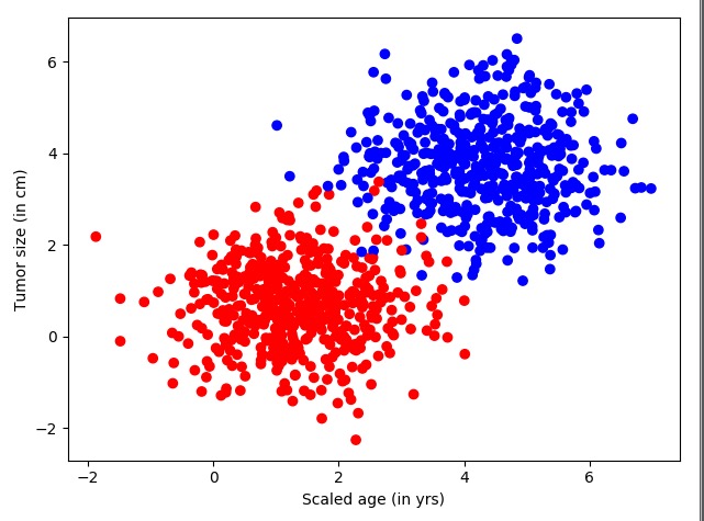
图中左下是红色的样本数据,右上是蓝色的样本数据。
2.构建网络结构
下面开始构建网络模型,见下方代码。使用前面刚刚学过的一个神经元,先定义输入、输出两个占位符,然后是w和b的权重。
代码7-1 线性逻辑回归(续)
## 构建网络结构
input_features = tf.placeholder(tf.float32, [None, input_dim])
input_labels = tf.placeholder(tf.float32, [None, lab_dim])

# 定义学习参数
W = tf.Variable(tf.random_normal([input_dim, lab_dim]), name="weight")
b = tf.Variable(tf.zeros([lab_dim]), name="bias")

output = tf.nn.sigmoid(tf.matmul(input_features, W) + b)  # 激活函数
cross_entropy = -(input_labels * tf.log(output) + (1 - input_labels) * tf.log(1 - output))  # 损失函数
ser = tf.square(input_labels - output)
loss = tf.reduce_mean(cross_entropy)
err = tf.reduce_mean(ser)
optimizer = tf.train.AdamOptimizer(0.04)
# 尽量用这个,因其收敛快,会动态调节梯度
train = optimizer.minimize(loss)   # 优化器
- 激活函数使用的是Sigmoid。
- 损失函数loss仍然使用交叉熵,里面又加了一个平方差函数,用来评估模型的错误率。
- 优化器使用AdamOptimizer。
3.设置参数进行训练
然后整个数据集迭代50次,每次的minibatchsize取25条。
代码7-1 线性逻辑回归(续)
maxEpochs = 50
minibatchSize = 25

# 启动session
with tf.Session() as sess:
    sess.run(tf.global_variables_initializer())

    for epoch in range(maxEpochs):
        sumerr = 0
        for i in range(np.int32(len(Y) / minibatchSize)):
            x1 = X[i * minibatchSize:(i + 1) * minibatchSize, :]
            y1 = np.reshape(Y[i * minibatchSize:(i + 1) * minibatchSize], [-1, 1])
            tf.reshape(y1, [-1, 1])
            _, lossval, outputval, errval = sess.run([train, loss, output, err],
                                                     feed_dict={input_features: x1, input_labels: y1})
            sumerr = sumerr + errval

        print("Epoch:", '%04d' % (epoch + 1), "cost=", "{:.9f}".format(lossval), "err=",
              sumerr / np.int32(len(Y) / minibatchSize))
每一次的计算都会将err错误值累加起来,数据集迭代完一次会将err的错误率进行一次平均,平均值再输出来。运行上面的代码,生成如下信息:
Epoch: 0001 cost= 0.937670827 err= 0.857066742182
Epoch: 0002 cost= 0.576581895 err= 0.474182988405
Epoch: 0003 cost= 0.326138794 err= 0.273106197715
……
Epoch: 0048 cost= 0.028127037 err= 0.019222549072
Epoch: 0049 cost= 0.027764326 err= 0.0191760268845
Epoch: 0050 cost= 0.027415426 err= 0.0191324938528
经过50次的迭代,得到了错误率为0.019的模型。
4.数据可视化
为了直观地解释线性可分,下面将模型结果和样本以可视化的方式显示出来,前一部分是先取100个测试点,在图像上显示出来,接着将模型以一条直线的方式显示出来。
代码7-1 线性逻辑回归(续)
train_X, train_Y = generate(100, mean, cov, [3.0], True)
colors = ['r' if l == 0 else 'b' for l in train_Y[:]]
plt.scatter(train_X[:, 0], train_X[:, 1], c=colors)
x = np.linspace(-1, 8, 200)
y = -x * (sess.run(W)[0] / sess.run(W)[1]) - sess.run(b) / sess.run(W)[1]
plt.plot(x, y, label='Fitted line')
plt.legend()
plt.show()
如上代码,模型生成的z用公式可以表示为z=x1w1+x2*w2+b,如果将x1和x2映射到直角坐标系中的x和y坐标,那么z就可以被分为小于0和大于0两部分。当z=0时,就代表直线本身,令上面的公式中z等于零,就可以将模型转化成如下直线方程:
x2=-x1* w1/w2-b/w2,即:y=-x* (w1/w2)-(b/w2)
其中,w1、w2、b都是模型中的学习参数,带到公式中用plot显示出来。运行代码,生成结果如图所示。
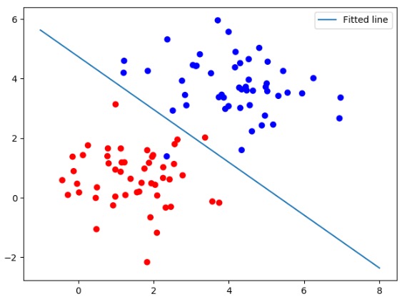
图7-2 线性逻辑回归
5.线性可分概念
如图7-2所示这种情况,可以用直线分割的方式解决问题,则可以说这个问题是线性可分的。同理,类似这样的数据集就可以被称为线性可分数据集合。凡是使用这种方法来解决的问题就叫做线性问题。
用线性逻辑回归处理多分类问题
还是接着前面的例子,这次在数据集中再添加一类样本,可以使用多条直线将数据分成多类。
构建网络模型完成将3类样本分开的任务。在实现过程中先生成3类样本模拟数据,构造神经网络,通过softmax分类的方法计算神经网络的输出值,并将其分开。
1.生成样本集
这里还使用上面代码中的generate函数,这次不同的是生成了2000个点、3类数据,并且使用one_hot编码。
代码7-2 线性多分类
import tensorflow as tf
import matplotlib.pyplot as plt
import numpy as np
from sklearn.utils import shuffle
# 对于上面的fit可以这么扩展变成动态的
from sklearn.preprocessing import OneHotEncoder

def onehot(y, start, end):
    ohe = OneHotEncoder()
    a = np.linspace(start, end - 1, end - start)
    b = np.reshape(a, [-1, 1]).astype(np.int32)
    ohe.fit(b)
    c = ohe.transform(y).toarray()
    return c


# 模拟数据点
def generate(sample_size, num_classes, diff, regression=False):
    np.random.seed(10)
    mean = np.random.randn(2)
    cov = np.eye(2)

    # len(diff)
    samples_per_class = int(sample_size / num_classes)

    X0 = np.random.multivariate_normal(mean, cov, samples_per_class)
    Y0 = np.zeros(samples_per_class)

    for ci, d in enumerate(diff):
        X1 = np.random.multivariate_normal(mean + d, cov, samples_per_class)
        Y1 = (ci + 1) * np.ones(samples_per_class)

        X0 = np.concatenate((X0, X1))
        Y0 = np.concatenate((Y0, Y1))
        # print(X0, Y0)

    if regression == False:  # one-hot  0 into the vector "1 0
        Y0 = np.reshape(Y0, [-1, 1])
        # print(Y0.astype(np.int32))
        Y0 = onehot(Y0.astype(np.int32), 0, num_classes)
        # print(Y0)
    X, Y = shuffle(X0, Y0)
    # print(X, Y)
    return X, Y


np.random.seed(10)

input_dim = 2
num_classes = 3
X, Y = generate(2000, num_classes, [[3.0], [3.0, 0]], False)
aa = [np.argmax(l) for l in Y]
colors = ['r' if l == 0 else 'b' if l == 1 else 'y' for l in aa[:]]
# 将具体的点依照不同的颜色显示出来
plt.scatter(X[:, 0], X[:, 1], c=colors)
plt.xlabel("Scaled age (in yrs)")
plt.ylabel("Tumor size (in cm)")
plt.show()
进行上面的代码,生成的结果如图所示。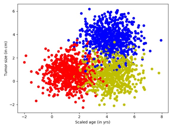
图7-3 三分类模拟数据集
在图7-3中,红色是原始的点,黄色点是在红色点的基础上将x+3.0后的变化,而蓝色的点是在红色点的基础上将x和y各加3.0。
2.构建网络结构
下面开始构建网络模型,这次使用了softmax分类,损失函数loss仍然使用交叉熵,对于错误率评估部分换成了取one_hot结果里面不相同的个数,优化器使用AdamOptimizer。
代码7-2 线性多分类(续)
lab_dim = num_classes
# tf Graph Input
input_features = tf.placeholder(tf.float32, [None, input_dim])
input_lables = tf.placeholder(tf.float32, [None, lab_dim])
# Set model weights
W = tf.Variable(tf.random_normal([input_dim, lab_dim]), name="weight")
b = tf.Variable(tf.zeros([lab_dim]), name="bias")
output = tf.matmul(input_features, W) + b

z = tf.nn.softmax(output)

a1 = tf.argmax(tf.nn.softmax(output), axis=1)  # 按行找出最大索引,生成数组
b1 = tf.argmax(input_lables, axis=1)
err = tf.count_nonzero(a1 - b1)  # 两个数组相减,不为0的就是错误个数

cross_entropy = tf.nn.softmax_cross_entropy_with_logits(labels=input_lables, logits=output)
loss = tf.reduce_mean(cross_entropy)  # 对交叉熵取均值很有必要

optimizer = tf.train.AdamOptimizer(0.04)  # 尽量用这个--收敛快,会动态调节梯度
train = optimizer.minimize(loss)  # let the optimizer train
3.设置参数进行训练
本次同样设置数据集迭代50次,每次的minibatchSize取25条。
代码7-2 线性多分类(续)
# 启动session
with tf.Session() as sess:
    sess.run(tf.global_variables_initializer())

    for epoch in range(maxEpochs):
        sumerr = 0
        for i in range(np.int32(len(Y) / minibatchSize)):
            x1 = X[i * minibatchSize:(i + 1) * minibatchSize, :]
            y1 = Y[i * minibatchSize:(i + 1) * minibatchSize, :]
            _, lossval, outputval, errval = sess.run([train, loss, output, err],
                                                     feed_dict={input_features: x1, input_lables: y1})
            sumerr = sumerr + (errval / minibatchSize)

        print("Epoch:", '%04d' % (epoch + 1), "cost=", "{:.9f}".format(lossval), "err=", sumerr / minibatchSize)
在迭代训练时对错误率的收集与前面的代码一致,每一次的计算都会将err错误值累加起来,数据集迭代完一次会将err的错误率进行一次平均,然后再输出平均值。运行上面的代码生成如下信息:
Epoch: 0001 cost= 0.408920079 err= 0.8544
Epoch: 0002 cost= 0.337683767 err= 0.3648
Epoch: 0003 cost= 0.321038276 err= 0.3328
Epoch: 0004 cost= 0.319500208 err= 0.32
……
Epoch: 0048 cost= 0.422929078 err= 0.2784
Epoch: 0049 cost= 0.423131853 err= 0.2784
Epoch: 0050 cost= 0.423317522 err= 0.2784
4.数据可视化
接下来一起看看对于三分类问题,线性可分是怎么分的。先取200个测试的点,在图像上显示出来,接着将模型中x1、x2的映射关系以一条直线的方式显示出来。因为输出端有3个节点,所以相当于是3条直线。
代码7-2 线性多分类(续)
    train_X, train_Y = generate(200, num_classes, [[3.0], [3.0, 0]], False)
    aa = [np.argmax(l) for l in train_Y]
    colors = ['r' if l == 0 else 'b' if l == 1 else 'y' for l in aa[:]]
    plt.scatter(train_X[:, 0], train_X[:, 1], c=colors)

    x = np.linspace(-1, 8, 200)

    y = -x * (sess.run(W)[0][0] / sess.run(W)[1][0]) - sess.run(b)[0] / sess.run(W)[1][0]
    plt.plot(x, y, label='first line', lw=3)

    y = -x * (sess.run(W)[0][1] / sess.run(W)[1][1]) - sess.run(b)[1] / sess.run(W)[1][1]
    plt.plot(x, y, label='second line', lw=2)

    y = -x * (sess.run(W)[0][2] / sess.run(W)[1][2]) - sess.run(b)[2] / sess.run(W)[1][2]
    plt.plot(x, y, label='third line', lw=1)

    plt.legend()
    plt.show()
    print(sess.run(W), sess.run(b))
运行上面的代码,输出如下,得到结果如图所示。
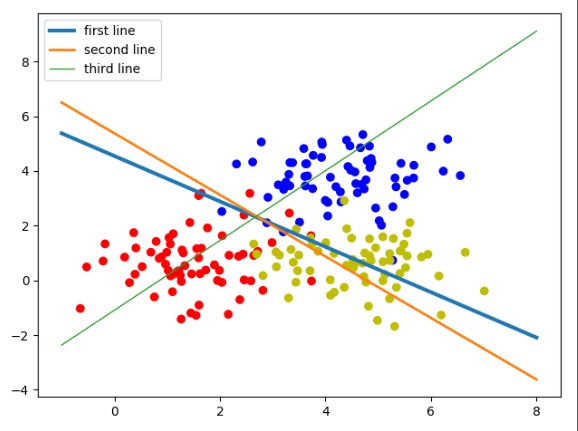
图为 三分类线性模型
[[-1.29152238 1.68322766 1.79681265]
[-0.55652267 2.47718096 -0.54918939]] [ 6.61509657 -8.44192219 -1.66505146]
图中,3个权重分别代表了3条线。还原成模型就是模型里3个输出的分类节点:
- 第1个输出节点代表分类0,红色,蓝线(first line)。
- 第2个输出节点代表分类1,蓝色,绿线(second line)。
- 第3个输出节点代表分类2,黄色,红线(third line)。
这3条直线的斜率和截距是由神经网络的学习参数转化而来的。在神经网络里,一个样本通过这3个公式会得到3个结果,这3个结果可以理解成3个类的特征值。其中哪个值最大,则表示该样本具有哪种类别的特征最强烈,即属于哪一类。可以在横轴随便找一个值,分别带到3条直线的公式里,哪条直线得出的y值最大,则说明该点属于哪一类。这3条线也没有把集合点分开,这是因为它们的分类规则是不一样的。下面回顾一下直线公式:
y=-x* (w1/w2)-(b/w2)
正常来讲:如果一个点在直线上,等式成立;如果点在直线的上方,那么左边的y值就大;如果点在直线的下方,那么右边的算式值就大。
但放到模型里对应的图像上并不是这样的,还取决于w1的正负取值,当w1为负时正好是相反的情况。从上例中的输出结果里可以看到,只有第一条线(蓝线)的w1是负数,所以蓝线是取其下面的点,红线和绿线是取其上方的点。举例:取一点红色的数据,如图所示。
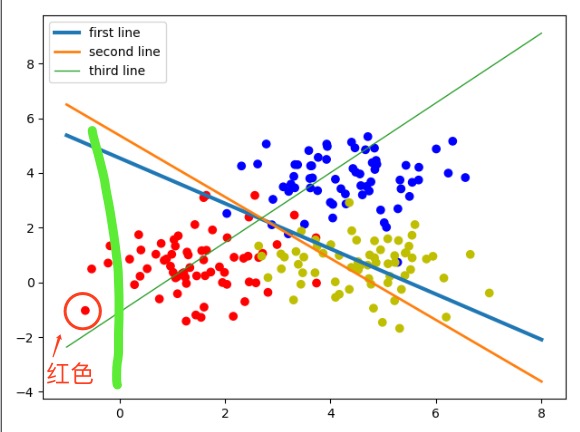
图 三分类线性模型分析
沿着y轴的方向平行画一条线经过该点,可以看到它在第一条线(蓝线)的下方,并且离蓝线的距离是最远的,所以它就属于第一条线对应的红色分类。说明对于这类的数据集,仍然可以使用线性可分的方法将其分开。本例也展示了线性可分在多分类问题上的应用与原理。
5.模型可视化
前面介绍了线性与模型的关系,现在把整个坐标系放到模型里,会得到一个更直观的模型分类可视化。为了方便演示,还是在图像上生成200个点并显示出来。然后按照坐标系的排列,把x1,x2放到模型里,见如下代码。
代码7-2 线性多分类(续)
    train_X, train_Y = generate(200, num_classes, [[3.0], [3.0, 0]], False)
    aa = [np.argmax(l) for l in train_Y]
    colors = ['r' if l == 0 else 'b' if l == 1 else 'y' for l in aa[:]]
    plt.scatter(train_X[:, 0], train_X[:, 1], c=colors)

    nb_of_xs = 200
    xs1 = np.linspace(-1, 8, num=nb_of_xs)
    xs2 = np.linspace(-1, 8, num=nb_of_xs)
    xx, yy = np.meshgrid(xs1, xs2)  # 创建网格
    # 初始化和填充 classification plane
    classification_plane = np.zeros((nb_of_xs, nb_of_xs))
    for i in range(nb_of_xs):
        for j in range(nb_of_xs):
            classification_plane[i, j] = sess.run(a1, feed_dict={input_features: [[xx[i, j], yy[i, j]]]})

    # 创建 color map 用于显示
    cmap = ListedColormap([
        colorConverter.to_rgba('r', alpha=0.30),
        colorConverter.to_rgba('b', alpha=0.30),
        colorConverter.to_rgba('y', alpha=0.30)])
    # 图示各个样本边界
    plt.contourf(xx, yy, classification_plane, cmap=cmap)
    plt.show()
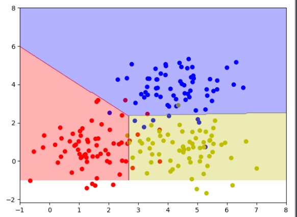
上面代码的运行结果如图7-6所示。将三分类模型用了不同的颜色区域进行区分,这样就是符合人眼规律的一个比较直观的可视化图样了。
图7-6 三分类模型可视化
认识非线性问题
在明白了线性问题之后,接着介绍非线性问题。非线性问题,就是用直线分不开的问题。为了解释这个概念,先来看一个数据集异或形态的数据,如图7-7所示。图7-7中只有4个点,蓝色为一类,红色一类,蓝色两个点的连线与红色两个点的连线会相交。对于这样的数据,你会发现无法使用一条直线将红色和蓝色两种类型的点分开,这就是非线性数据。
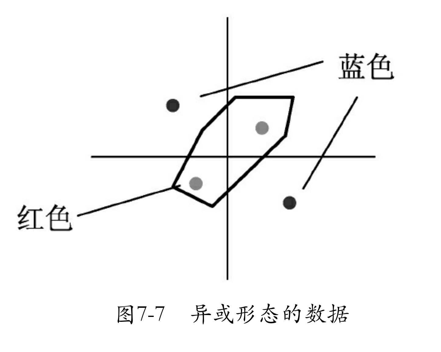
对于这样的数据,有一种笨方法,即对原始数据变形,使其变为线性分布。例如,将数据x1、x2进行一次绝对值运算,这时数据就会变为如图7-8所示的样子。
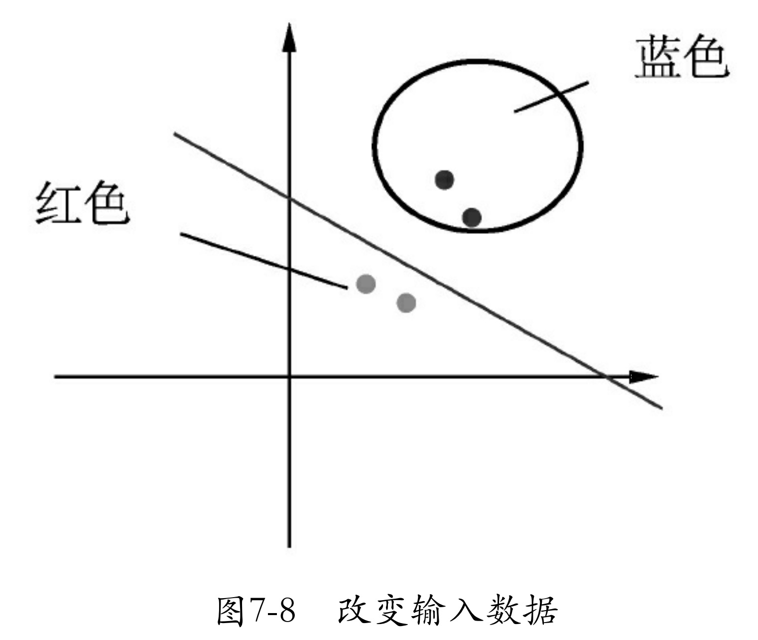
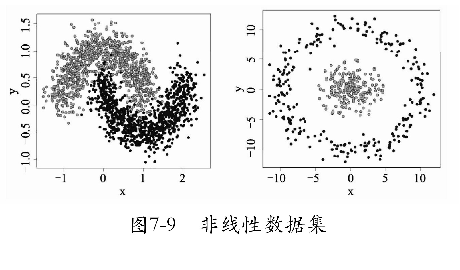
类似图7-8的方法有很多种,还可以将其进行一次平方运算。但这一切都是在人们肉眼看到模型分布后,通过分析得来的。而实际应用中会遇到更复杂的非线性数据集(如图7-9所示),或者有时数据维度太大,根本无法可视化。这时就需要用一种新方法 —— 多层神经网络 来解决问题了。